Z-Table Foundations: Demystifying Probability Density & Cumulative Functions
Ever gazed at a Z-Table, those meticulously organized grids of numbers, and wondered about the intricate mathematical machinery that brings them into existence? While statisticians and data analysts routinely rely on these tables for quick insights into normal distributions, understanding their origins reveals the elegant interplay of fundamental statistical concepts: the Probability Density Function (PDF) and the Cumulative Distribution Function (CDF). These two functions are the bedrock upon which the entire utility of the Z-Table rests, allowing us to translate raw data into meaningful probabilities and percentile ranks.
At its heart, the Z-Table is a practical tool derived from the theoretical elegance of the normal (or Gaussian) distribution. This ubiquitous bell-shaped curve describes many natural phenomena and datasets, from human heights to measurement errors. But to move from a theoretical curve to concrete probabilities, we need the power of functions that can quantify likelihood over continuous ranges. Let's delve into how the PDF and CDF achieve this, laying the essential groundwork for understanding Mastering Z-Scores: Understanding Table Calculation & Use.
Unveiling the Probability Density Function (PDF)
The journey begins with the Probability Density Function (PDF). In probability theory, the PDF of a continuous random variable provides a way to describe the relative likelihood for the variable to take on a given value. Unlike discrete variables, where we can talk about the exact probability of a specific outcome (e.g., rolling a 3 on a die), a continuous variable has an infinite number of possible values within any given range. This means the absolute probability of it taking on *any single specific value* is, mathematically speaking, zero.
Consider a person's height. What's the probability someone is *exactly* 175.00000000 cm tall? It's infinitesimally small. Instead, the PDF allows us to calculate how much more likely it is for a random variable to fall within one interval compared to another. It helps us understand the "density" of probability around certain points. The higher the value of the PDF at a particular point, the more probable it is that the random variable will be near that point.
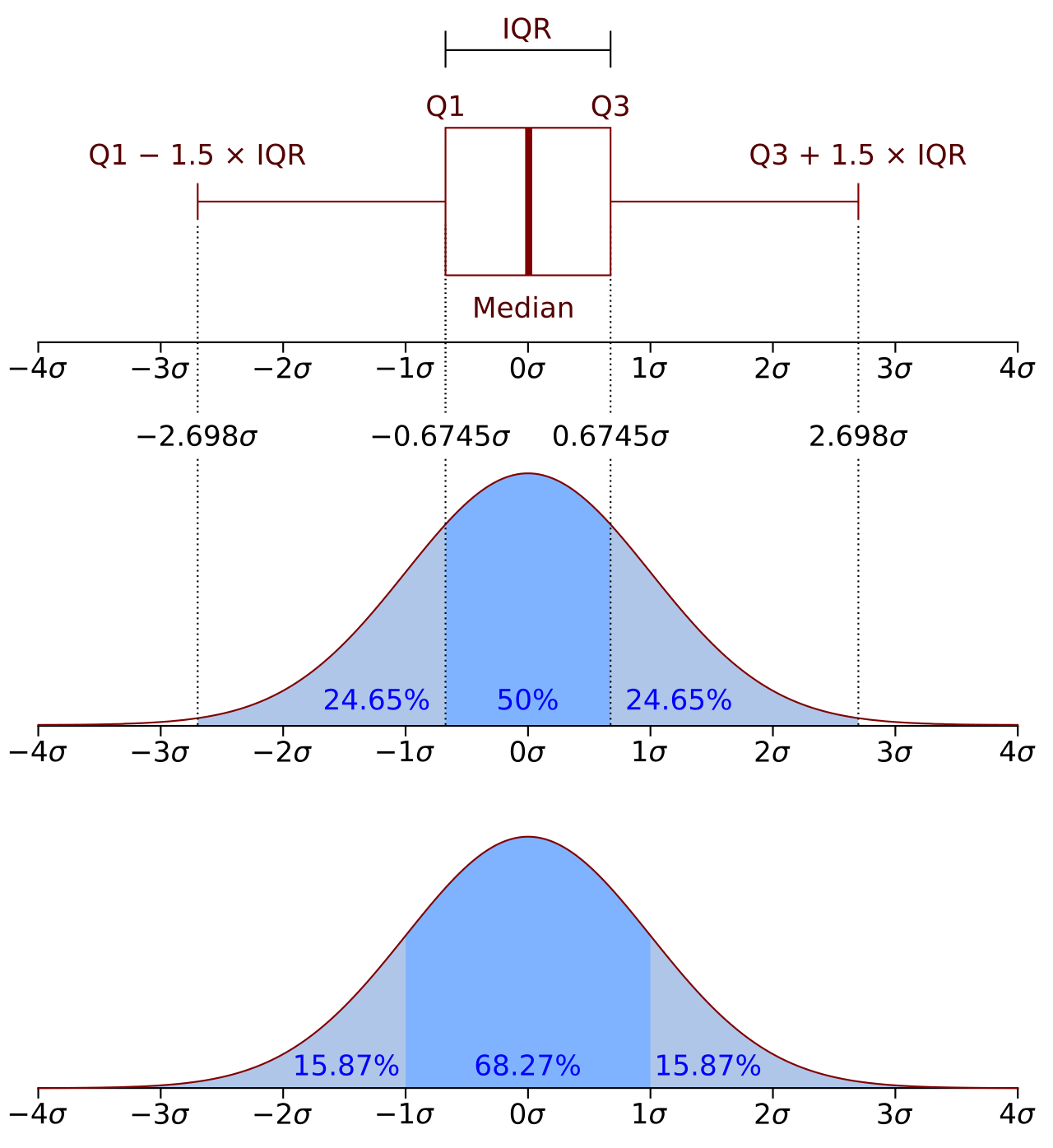
For a normal distribution, the PDF is characterized by its mean (μ) and standard deviation (σ). When graphed, this function produces the familiar bell-shaped curve, symmetric around its mean. The formula for the normal distribution's PDF is quite formidable:
f(x) = (1 / (σ * sqrt(2π))) * e^(-(x - μ)^2 / (2σ^2))
However, for the standard normal distribution – which is the basis for Z-Tables – the mean (μ) is 0 and the standard deviation (σ) is 1. This simplification yields a more manageable form of the PDF, whose graph is perfectly centered at zero and has a standard spread.
It's crucial to understand that the PDF itself does not give us probabilities directly. To find the actual probability that a variable falls within a certain range (e.g., between X1 and X2), we need to calculate the area under the PDF curve between those two points. This process requires integration, which leads us to our next critical function.
The Power of the Cumulative Distribution Function (CDF)
While the PDF gives us the probability density, the Cumulative Distribution Function (CDF) bridges the gap to actual probabilities. In essence, the CDF of a random variable X, evaluated at a point x, represents the probability that X will take a value less than or equal to x. It literally "accumulates" the probabilities from the far left tail of the distribution up to the point x.
Mathematically, the CDF is derived by integrating the PDF from negative infinity up to the point x. For a standard normal distribution, where the mean is 0 and the standard deviation is 1, the CDF is typically denoted as Φ(z) and can be expressed as:
Φ(z) = ∫(-∞ to z) f(t) dt
Where f(t) is the PDF of the standard normal distribution. This integration process is what transforms the density values into cumulative probabilities. When we calculate the CDF for various values of 'z' (which represent Z-scores – the number of standard deviations a value is from the mean), we obtain the very values that populate a standard Z-Table.
The CDF offers invaluable insights:
- Percentile Ranks: The value of the CDF at any given x directly corresponds to the percentile rank of that value. If Φ(z) = 0.85, it means that 85% of the data falls at or below that particular Z-score.
- Range Probabilities: To find the probability that a variable falls between two values (e.g., between z1 and z2), we simply subtract their respective CDF values: P(z1 ≤ Z ≤ z2) = Φ(z2) - Φ(z1).
- "Greater Than" Probabilities: To find the probability that a variable is greater than a certain value z, we use the complement rule: P(Z > z) = 1 - Φ(z).
The CDF effectively maps Z-scores to their corresponding probabilities, providing a complete picture of how probabilities accumulate across the distribution.
From Functions to the Z-Table: A Practical Bridge
Now we arrive at the Z-Table itself, the practical manifestation of the CDF for the standard normal distribution. Each entry in a standard Z-Table represents the cumulative probability (the area under the curve) from negative infinity up to a specific Z-score. The rows and columns typically represent the Z-score to one or two decimal places, making it easy to look up values.
The creation of a Z-Table from scratch involves performing the complex integration of the standard normal PDF for a vast range of Z-score values. This is not a trivial calculation and historically required significant computational effort. While it's certainly possible to generate these values using modern software like Python, as explored in How to Create a Z Score Table from Scratch, it's generally an inefficient and unnecessary exercise for everyday statistical analysis. The beauty of pre-made Z-Tables lies in their efficiency; they allow us to bypass these arduous calculations and directly access the probabilities we need.
Understanding the Z-Table's foundations in PDF and CDF empowers us to:
- Interpret Z-scores meaningfully: A Z-score isn't just a number; it tells us how many standard deviations away from the mean a data point lies, and the Z-Table tells us the probability associated with that deviation.
- Compare data from different distributions: By converting any normally distributed data into Z-scores, we standardize it, making direct comparisons possible regardless of original means or standard deviations.
- Make informed decisions: From quality control in manufacturing to assessing student performance, Z-scores and their associated probabilities are vital for making statistically sound judgments.
Conclusion
The Z-Table is more than just a grid of numbers; it's a powerful statistical instrument built upon the robust theoretical frameworks of the Probability Density Function and the Cumulative Distribution Function. The PDF describes the relative likelihood across a continuous range, while the CDF accumulates these likelihoods into tangible probabilities, mapping values to their percentile ranks. This journey from abstract mathematical functions to a practical, pre-calculated table underscores the ingenuity in statistical science. By appreciating these foundations, we not only gain a deeper understanding of the Z-Table's utility but also enhance our ability to interpret data, quantify uncertainty, and make more data-driven decisions across various fields.